Microsoft Excel - Pivot tables

Learn about Pivot tables

What is a Pivot table?

A Pivot table is an interactive way to quickly summarize large amounts of data. Use a Pivot table report to analyze numeric data in detail and to answer unanticipated questions about your data.

A Pivot table is especially designed for:

• Querying large amounts of data in many user-friendly ways.
• Subtotaling and aggregating numeric data, summarizing data by categories and subcategories, and creating custom calculations and formulas.
• Expanding and collapsing levels of data to focus your results, and drilling down to details from the summary data for areas that are of interest to you.
• Moving rows to columns or columns to rows (or "pivoting") to see different summaries of the source data.
• Filtering, sorting, grouping, and conditionally formatting the most useful and interesting subset of data to enable you to focus on the information that you want.
• Presenting concise, attractive, and annotated online or printed reports.

You often use a Pivot table when you want to analyze related totals, especially when you have a long list of figures to sum, and aggregated data or subtotals would help you look at the data from different perspectives and compare figures of similar data.

Click to download the example file.

Creating a Pivot table from worksheet data

1. To use data in an Excel table as the data source, click a cell inside the Excel table.
   Note: Make sure that the range has column headings or that headers are displayed in the table, and that there are no blank rows in the range or table.
2. On the Insert tab, in the Tables group, click PivotTable.
   

   
   

   
   

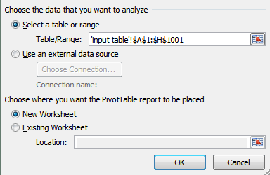
   Excel displays the Create PivotTable dialog box.

   
   

   
   
3. Under Choose the data that you want to analyze, make sure that Select a table or range is selected, and then in the Table/Range box, verify the range of cells that you want to use as the underlying data.
   
   Excel automatically determines the range for the PivotTable report, but you can replace it by typing a different range or a name that you defined for the range.
   
   Tip: You can also click Collapse Dialog to temporarily hide the dialog box, select the range on the worksheet, and then click Expand Dialog .


4. Under Choose where you want the PivotTable report to be placed, specify a location by doing one of the following:
   • To place the PivotTable report in a new worksheet starting at cell A1, click New Worksheet.
   
   
   • To place the PivotTable report in an existing worksheet, select Existing Worksheet, and then in the Location box, specify the first cell in the range of cells where you want to position the Pivot table.


5. Click OK.
   
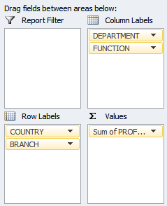
   Excel adds an empty Pivot table to the specified location and displays the PivotTable Field List so that you can add fields, create a layout, and customize the Pivot table.


6. To add fields to the report, do one or more of the following:
   
   
   • To place a field in the default area of the layout section, select the check box next to the field name in the field section.

     
     

     
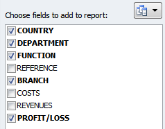
     By default, nonnumeric fields are added to the Row Labels area, numeric fields are added to the Values area, and Online Analytical Processing (OLAP) date and time hierarchies are added to the Column Labels area.
   
   
   • To place a field in a specific area of the layout section, right-click the field name in the field section, and then select Add to Report Filter, Add to Column Label, Add to Row Label, or Add to Values.
   
   
   • To drag a field to the area that you want, click and hold the field name in the field section, and then drag it to an area in the layout section.

     
     

Click to download the example file.